Why Is Business Investment Sluggish: An Alternative View to Alan Kohler

On ABC News on Sunday night, Alan Kohler in his regular spot showed how business investment, especially in plant and equipment, has  been sluggish for the past several years.  Despite acknowledging a number of theories, of course he blamed it on the lack of a coherent bi-partisan climate policy- his favourite hobby-horse.

Time for a reality check.

Firstly, Figure 1 shows the Australian All Ordinaries Index with the key dates of proposal, adoption, deferral, re-proposal, and eventual scrapping of all versions of carbon tax, with the 2014 and 2019 elections when Labor’s climate dreams were roundly rejected.  It is important to realise that various Federal and State renewable energy incentives have also been introduced during this time.

Figure 1:  All Ordinaries Index 2007-2022 (per Westpac)

The share market seems to have been largely oblivious to climate policy.  What about business investment?

I checked the recently released ABS data, here and here.

Alan Kohler used 3 data points (decadal annual growth rates).  I looked at the 124 quarterly values of private investment in 2021 dollar values, from March 1991 to December 2021.

Figure 2:  Quarterly Private Capital Investment, 1991-2021

While Construction boomed from 2011 to 2015, it is true that investment in plant, equipment, and machinery has barely moved since 2010.

These categories can be further broken down into Mining and all others except for mining:

Figure 3:  Capital Investment in Construction, Mining and Non-mining

That big bump was the mining boom, which also shows but to a lesser extent in investment in Plant and Equipment:

Figure 4:  Capital Investment in Plant & Equipment, Mining and Non-mining

Note that the total figure for Plant and equipment is nearly all from non-mining activity.  Note the peak was reached in the December quarter of 2009, before the big reduction brought about by the GFC of 2008 and 2009.

Rather than annual growth or actual quarterly investment, an alternative comparison is with GDP.

Figure 5:  Australia’s Gross Domestic product

Despite the sluggish early 1990s, the GFC and the pandemic, GDP has been growing at an increasing rate, especially in the last five years.

Figure 6:  Quarterly Private Capital Investment as a percentage of GDP, 1991-2021

Mining investment in construction has been huge, and the economy has been reaping the benefit since 2016. 

Figure 7 shows investment in plant and equipment (which Alan Kohler says has been flat since 2011 as a result of not having certainty in climate policy) outside the mining industry.  The dates from Figure 1 are shown.

Figure 7:  Quarterly Plant and Equipment Investment as a percentage of GDP, 1991-2021

Alan Kohler’s explanation is obviously wrong. Perhaps he could explain why plant and equipment expenditure relative to GDP has been steadily decreasing since 1996- well before any mention of climate policy.  That would seem to be a much more serious problem.

But I don’t think he will- there’s an election coming up.

How Unusual Is All This Rain We’ve Had?

Yesterday, 2^nd March, ABC weather reporter Kate Doyle posed this question on the ABC website about the recent rain event in SE Queensland and Northern NSW.

Her answer to the above question was:

“Very unusual.

The rainfall totals from this event have been staggering. 

From 9am Thursday to 9am Monday three stations recorded over a metre of rain:

– 1637mm at Mount Glorious, QLD 
– 1180mm at Pomona, QLD
– 1094mm at Bracken Ridge “

She goes on to say:  “South-east Queensland and northern NSW are historically flood prone and have certainly flooded before but this event is definitely different from those we have seen in the past.”  And of course climate change is involved.

Time for a reality check. 

My answer to Kate’s question:  Not very unusual at all.

I went looking at Climate Data Online for four day rainfall totals over one metre, to compare with the recent totals above at Mount Glorious, Pomona, and Bracken Ridge. 

For a start, Pomona’s BOM station has been closed for years, and Bracken Ridge is not listed at all, so those reports are from rain gauges external to the BOM network and can’t be checked. 

That’s OK.  In about half an hour I found the following four day rainfall records.

Crohamhurst	4/2/1893	1963.6mm
Yandina	3/2/1893	1597.8mm
Tully Sugar Mill	13/02/1927	1421.3mm
Palmwoods	4/2/1893	1244.6mm
Buderim	3/2/1893	1150.3mm
Bloomsbury	20/01/1970	1141.8mm
Dalrymple Heights	6/04/1989	1141mm
Innisfail	3/04/1911	1075.8mm
Nambour	11/1/1898	1013mm

1893 was a wet year!  Crohamhurst had 2023.8 in five days, and Brisbane had three floods in two weeks in February and another in June.

And there is no such thing as a “rain bomb”, a term invented to make it sound unprecedented.  This was an entirely natural and normal rain event.  Slow moving tropical lows drift south every few years in the wet season, producing a large proportion of Queensland’s average rainfall.

Floods have affected Brisbane and surrounds since before European settlement.  The Bureau has an excellent compilation of accounts of past floods at

http://www.bom.gov.au/qld/flood/fld_history/brisbane_history.shtml

It includes this graphic showing the height of known floods.  I have added an indication of the height of the 2022 flood.

Here are some notable Brisbane floods:

1825       a flood probably as high as the 1893 flood

1841       8.43m

1844       about1.2 metres lower than 1841

1864       ?

1887       ?

1889       ?

1890       ?

1893       8.35m

“              8.09m

“              ?

“              ?

1908       4.48m

1974       5.45m

2011       4.46m

2022       3.85m

Every flood is different- water backs up higher in unexpected places, or gets away faster, so for many people this flood was worse than 2011.  However it is beyond any doubt that this flood, heartbreaking as it was for many people, could have been much worse.  It was nowhere near as big as several in the past.  Wivenhoe Dam worked as planned this time, which greatly lessened the impact.

Another thing worth remembering:  floods were more frequent and higher in the 19^th Century than they have been in the last 100 years.

ABC journalists need to do a lot more research.

More Evidence That The Australian Temperature Record Is Complete Garbage

The Bureau of Meteorology is either incompetent or has knowingly allowed inaccurate data to garble the record.

My colleague Chris Gillham at http://www.waclimate.net/ has alerted me to growing problems with the BOM’s record for Diurnal Temperature Range (DTR).  DTR is the difference between daytime temperature (Tmax) and night-time temperature (Tmin). 

According to Dr Karl Braganza’s paper at https://agupubs.onlinelibrary.wiley.com/doi/10.1029/2004GL019998 , “an index of climate change” is that DTR should decrease as greenhouse gases accumulate. To oversimplify, greenhouse gases will enhance daytime temperature while at night greenhouse gases will slow down cooling.  With increasing greenhouse gas concentration, daytime maxima are expected to increase, certainly, but the effect on night-time minima will be relatively greater.  Thus, minimum temperatures will increase faster than maxima, and DTR will decrease.  While Dr Braganza was referring to global values, Australia is a large dry continent where DTR should show up clearly.

We now have 111 years of temperature data in ACORN-SAT (Australian Climate Observation Reporting Network- Surface Air Temperatures).  In this post I only use Acorn temperature data and corresponding rainfall data.  Skeptics have been bagging Acorn ever since it was introduced, and for good reasons as you will see.

Figure 1 is straight from the Bureau’s climate time series page, and shows how DTR has varied over the years.  There is a centred 15 year running mean overlaid. 

Figure 1: Official plot of annual DTR

Melbourne, We Have A Problem… DTR has been increasing recently.

I have used BOM data to make plots that show this more clearly.  First, Figure 2 shows annual DTR from 1910 to 2020 has no trend.  It should be decreasing.

Figure 2:  Annual DTR

There appears to be a distinct step up around 2000-2002.

Figure 3 shows the same data for the last 70 years, broken into two periods, from 1951 to 2000, and 2001 to 2020.

Figure 3:  DTR since 1951

From 1951 to 2000, DTR behaves as it should, with a long term decrease.  After 2000, DTR steps up well above expected values.  The average from 1981-2000 is -0.12 C.  From 2001-2020 the average is +0.35C.  DTR suddenly increases by nearly 0.5C. Why?

DTR is very much governed by that other greenhouse gas, H2O.  Dry days, months and years produce hot days and cooler nights; wet periods result in cooler than average days and warmer than average nights.  This relationship is shown in Figure 4.

Figure 4:  DTR anomalies plotted against rainfall anomalies- all years 1910-2020

As rainfall increases, DTR decreases.  The effect is more marked in very wet (>100mm above average) and very dry (100mm or more below average) years.

Figure 5 shows time series of DTR (as in Figure 2) and rainfall.  Rainfall has been inverted and scaled down by a factor of 250.

Figure 5:  DTR and Inverted, Scaled Rainfall

There is close match between the two.

Using 10 year averages in Figure 6 makes the change after 2001 much clearer.

Figure 6:  Decadal means of DTR and inverted, scaled rainfall

The 10 year average rainfall to 2020 is about the same as the 1961-1990 average (the period the BOM uses for calculating anomalies).  The 10 year average DTR should be about the same value- not at a record level.

As DTR decrease due to greenhouse gas accumulation is caused by minimum temperatures increasing faster than maximum temperatures, Figure 7 shows 10 year averages of maxima and minima for all years to 2020.

Figure 7:  10 year running means of Tmax and Tmin

Tmax has clearly accelerated in the last 20 years, increasing much faster than Tmin.

This is NOT what should be happening: indeed it is the exact opposite of what greenhouse theory predicts.

Something happened to Australian maximum temperature recording or reporting early this century.  I suspect that the BOM changed from using the highest one-minute average of temperatures recorded in Automatic Weather Systems to the current highest one-second value for the day becoming the reported maximum; or else the design of a significant number of AWS changed, with new, faster-responding probes replacing old ones.

I also suspect I know why this was allowed to happen and continue.

Warmer minimum temperatures at night and in winter are not very scary, but record high temperatures and heatwaves make headlines.

It would suit the Global Warming Enthusiasts in the Bureau for apparently rapidly rising maxima and ever higher records being broken to make headlines, frighten the public, put pressure on governments, and generally support The Narrative.

But someone forgot to tell the left hand what the right hand was doing.

The result is that they are now faced with a contradiction- Diurnal Temperature Range is not decreasing as it should. 

The Bureau is either incompetent or has knowingly allowed inaccurate data to garble the record.

The World’s Biggest Thermometer

Are temperatures today unprecedented and dangerously high?  Apparently- the IPCC’s 6^th Assessment Report says that current temperatures are higher than at any time in the last 125,000 years

But that is wrong.  Temperatures today are cooler than they were in the past.

In making that statement I am not referring to data from ice cores (as in my previous posts here and here), but a simple and accessible temperature measurement device: the biggest thermometer in the world.

The following statements are uncontroversial:

1 Sea level rise is largely due to melting of glaciers and thermal expansion of the oceans.

2 Thermal expansion and glacial melting are symptoms of temperature increase.

3 Higher sea level indicates warmer conditions, lower sea level indicates colder conditions.

4 Sea levels are currently rising (by a small amount- NOAA says Fort Denison, Sydney, has a rise of 0.65mm per year).

5 This indicates temperatures have been rising.

6 But sea levels and therefore temperatures were higher than now about 4,000 to 7,000 years ago.

If you doubt point 6, you can easily tell whether it was warmer or cooler in the past relative to today.

How?  By looking for evidence of sea level change in areas that are not affected by tectonic rising or falling coastal land, or by large scale water run off or glacial melting, or by very large underground water extraction.

Areas such as the eastern coastline of Australia- the world’s biggest thermometer.

The continent of Australia is very old and flat.  It is in the middle of its continental plate with very little tectonic activity.  Australia’s coastlines are therefore largely stable with little vertical movement, apart from a small tilt down at the northern edge and a small uplift along the southern coast.  Australia is also a very long way from ancient ice sheets.

Evidence of higher sea level is plain to see in many places around Australia.  For example, at Phillip Island in Victoria, Victorian Resources Online describes raised Holocene beaches at Chambers Point, 0.5m and 3 to 5m above high water mark.  Arrows on this Google Maps image show where to find them.

More evidence at Wooloweyah Lagoon, near Maclean in NSW:

And Bulli, NSW:

There are many, many other locations where you can find Holocene beaches well above current sea level. 

Some of the height of these stranded beaches is probably due to the weight of deeper seawater from the melting ice sheets gradually tilting up continental coastlines as the sea floor deepened leading to an apparent drop in sea level at the coast.  However, as Lewis et al (2013) and Sloss et al (2018) (see Appendix below) show, this was of lesser importance especially in northern Australia.  Sea level fall was largely due to climatic influences- in particular, cooling and drying since the Holocene Optimum.

To conclude:  Sea levels were higher in the past, so temperatures must have been higher. 

Therefore there is no evidence that current temperature rise is anything unusual.  Just check the world’s biggest thermometer.

Appendix:  Here are a few of many references to higher Australian sea levels in the Holocene, and reasons for variation.

Sloss et al (2007)  Holocene sea-level change on the southeast coast of Australia: a review

“Present sea level was attained between 7900 and 7700 cal. yr BP, approximately 700—900 years earlier than previously proposed. Sea level continued to rise to between +1 and +1.5 m between 7700 and 7400 cal. yr BP, followed by a sea-level highstand that lasted until about 2000 cal. yr BP followed by a gradual fall to present. A series of minor negative and positive oscillations in relative sea level during the late-Holocene sea-level highstand appear to be superimposed over the general sea-level trend.”

ABC TV catalyst 19/6/2008

Even the ABC says sea levels were higher in the Holocene!

Lewis et al (2008) Mid‐late Holocene sea‐level variability in eastern Australia

“We demonstrate that the Holocene sea-level highstand of +1.0–1.5 m was reached ∼7000 cal yr bp and fell to its present position after 2000 yr bp.”

Moreton Bay Regional Council, Shoreline Erosion Management Plan for Bongaree, Bellara, Banksia Beach and Sandstone Point (2010)

“Sea levels ceased rising about 6,500 years ago (the Holocene Stillstand) when they reached approximately 0.4 to 1m above current levels. By 3,000 years before present they had stabilised at current levels”

Switzer et al (2010) Geomorphic evidence for mid–late Holocene higher sea level from southeastern Australia

“This beach sequence provides new evidence for a period of higher sea level 1–1.5 m higher than present that lasted until at least c. 2000–2500 cal BP and adds complementary geomorphic evidence for the mid to late Holocene sea-level highstand previously identified along other parts of the southeast Australian coast using other methods.”

Lewis et al (2013) Post-glacial sea-level changes around the Australian margin: a review

“The Australian region is relatively stable tectonically and is situated in the ‘far-field’ of former ice sheets. It therefore preserves important records of post-glacial sea levels that are less complicated by neotectonics or glacio-isostatic adjustments. Accordingly, the relative sea-level record of this region is dominantly one of glacio-eustatic (ice equivalent) sea-level changes. ….Divergent opinions remain about: (1) exactly when sea level attained present levels following the most recent post-glacial marine transgression (PMT); (2) the elevation that sea-level reached during the Holocene sea-level highstand; (3) whether sea-level fell smoothly from a metre or more above its present level following the PMT; (4) whether sea level remained at these highstand levels for a considerable period before falling to its present position; or (5) whether it underwent a series of moderate oscillations during the Holocene highstand.”

Leonard et al (2015) Holocene sea level instability in the southern Great Barrier Reef, Australia: high-precision U–Th dating of fossil microatolls

“RSL (relative sea level) was as least 0.75 m above present from ~6500 to 5500 yr before present (yr BP; where “present” is 1950). Following this highstand, two sites indicated a coeval lowering of RSL of at least 0.4 m from 5500 to 5300 yr BP which was maintained for ~200 yr. After the lowstand, RSL returned to higher levels before a 2000-yr hiatus in reef flat corals after 4600 yr BP at all three sites. A second possible RSL lowering event of ~0.3 m from ~2800 to 1600 yr BP was detected before RSL stabilised ~0.2 m above present levels by 900 yr BP. While the mechanism of the RSL instability is still uncertain, the alignment with previously reported RSL oscillations, rapid global climate changes and mid-Holocene reef “turn-off” on the GBR are discussed.”

Sloss et al (2018) Holocene sea-level change and coastal landscape evolution in the southern Gulf of Carpentaria, Australia

“ By 7700 cal. yr BP, sea-level reached present mean sea-level (PMSL) and continued to rise to an elevation of between 1.5 m and 2 m above PMSL. Sea level remained ca. + 1.5 between 7000 and 4000 cal. yr BP, followed by rapid regression to within ± 0.5 m of PMSL by ca. 3500 cal. yr BP. When placed into a wider regional context results from this study show that coastal landscape evolution in the tropical north of Australia was not only dependent on sea-level change but also show a direct correlation with Holocene climate variability….  Results indicate that Holocene sea-level histories are driven by regional eustatic driving forces, and not by localized hydro-isostatic influences. “

Dougherty et al (2019)  Redating the earliest evidence of the mid-Holocene relative sea-level highstand in Australia and implications for global sea-level rise

“The east coast of Australia provides an excellent arena in which to investigate changes in relative sea level during the Holocene…. improved dating of the earliest evidence for a highstand at 6,880±50 cal BP, approximately a millennium later than previously reported. Our results from Bulli now closely align with other sea-level reconstructions along the east coast of Australia, and provide evidence for a synchronous relative sea-level highstand that extends from the Gulf of Carpentaria to Tasmania. Our refined age appears to be coincident with major ice mass loss from Northern Hemisphere and Antarctic ice sheets, supporting previous studies that suggest these may have played a role in the relative sea-level highstand. Further work is now needed to investigate the environmental impacts of regional sea levels, and refine the timing of the subsequent sea-level fall in the Holocene and its influence on coastal evolution.”

Helfensdorfer et al (2020) Atypical responses of a large catchment river to the Holocene sea-level highstand: The Murray River, Australia

“Three-dimensional numerical modelling of the marine and fluvial dynamics of the lower Murray River demonstrate that the mid-Holocene sea-level highstand generated an extensive central basin environment extending at least 140 kilometres upstream from the river mouth and occupying the entire one to three kilometre width of the Murray Gorge. This unusually extensive, extremely low-gradient backwater environment generated by the two metre sea-level highstand….”

Climate Change in Context

In my last post I showed some plots of temperature data derived from ice cores at Vostok base in Antarctica, which indicate we are close to the end of the Holocene.

Here are some more plots from the same data so we can put present concerns about warming in some context.  Please remember- temperatures calculated from ice cores have a resolution of from 20 years recently to 40 to 50 years in the mid-Holocene, to 80 to 85 years in the glacial maximum.  Temperatures shown may be regarded as a rough average of conditions over those intervals.  Also note this dataset is for one point on the earth’s surface, not a global average.  Nevertheless it is a very important dataset as it shows polar conditions over a very long period.

Figure 1:  Vostok temperatures relative to 1999 over the last 20,000 years

The previous glacial maximum had temperatures in the Antarctic about 9 degrees colder than now.  This was followed by a strong warming, the Termination of glacial conditions, resulting in 11,000 years of warm conditions, the Holocene.  The Holocene was not uniformly warm but featured fluctuations of up to 2 degrees above and below current temperatures.  I will look at this later, but first I shall take a closer look at the Termination.  

Figure 2:  Vostok temperatures during the Termination

Point A marks the start of the Termination warming.  Temperatures rose from A to B (by about 6.5 degrees in 3,000 years- about 0.2 degrees per 100 years- so not exactly “rapid” warming).  Temperatures then fell about 2 degrees, before rising even more sharply from C to D, the start of the Holocene.  Figure 3 shows temperatures in this final part of the Termination.

Figure 3:  Vostok temperatures in the steepest part of the Termination

Temperatures increased by about 5 degrees over a bit more than 1,100 years.  Yes, the warming rate was indeed steeper- 0.44 degrees per 100 years on average.  However, the temperature rose 1 degree in less than 50 years at the end of this period.

During the Termination, long term temperature rise was gradual, but punctuated by short periods of much more rapid rise.

Now let’s look at temperature change in the Holocene.

Figure 4:  Vostok temperatures 7,000 to 9,000 years ago

Conditions were not uniformly warm, with fluctuations from -1 to +.5C relative to 1999 over hundreds of years.  But there was one episode with a rise of 2.93 degrees in less than 100 years- now that’s rapid warming.

Figure 5:  Vostok temperatures in the last 2,020 years

More recently, temperatures rose 1.94 degrees in 155 years to 1602, and again 2.2 degrees in 44 years to 1809.

You will notice I have shown 3 datapoints showing 21 year mean annual surface air temperatures at Vostok (1970, 1990, and 2010, with zero at 1990).  This is merely for interest- instrumental air temperatures should never be appended to ice core data.  What it does show is that the rate of present temperature change is well within the range of natural variation.

This is also evident when a Greenland ice core series is compared with modern surface air temperatures.

Figure 6:  Greenland (GISP2) temperatures in the last 4,000 years

I have inserted the decadal average of -29.9 C at the GISP borehole from 2001-2010.  Notice how unremarkable that is.

As the fluctuations at GISP and Vostok have been occurring for thousands of years something other than carbon dioxide emissions must be responsible.

So what about carbon dioxide? Data in the next figure is from Dome Fuji, also in Antarctica.

Figure 7:  Insolation, temperature, and CO2 in the last 350,000 years

Notice that at no time in previous interglacials did carbon dioxide concentration exceed 300ppm, (and despite the higher temperatures than now there was no “runaway” warming.)    And as the Carbon Dioxide Information Analysis Centre says

There is a close correlation between Antarctic temperature and atmospheric concentrations of CO₂ (Barnola et al. 1987). The extension of the Vostok CO₂ record shows that the main trends of CO₂ are similar for each glacial cycle. Major transitions from the lowest to the highest values are associated with glacial-interglacial transitions. During these transitions, the atmospheric concentrations of CO₂ rises from 180 to 280-300 ppmv (Petit et al. 1999). The extension of the Vostok CO₂ record shows the present-day levels of CO₂ are unprecedented during the past 420 kyr. Pre-industrial Holocene levels (~280 ppmv) are found during all interglacials, with the highest values (~300 ppmv) found approximately 323 kyr BP. When the Vostok ice core data were compared with other ice core data (Delmas et al. 1980; Neftel et al. 1982) for the past 30,000 – 40,000 years, good agreement was found between the records: all show low CO₂ values [~200 parts per million by volume (ppmv)] during the Last Glacial Maximum and increased atmospheric CO₂ concentrations associated with the glacial-Holocene transition. According to Barnola et al. (1991) and Petit et al. (1999) these measurements indicate that, at the beginning of the deglaciations, the CO₂ increase either was in phase or lagged by less than ~1000 years with respect to the Antarctic temperature, whereas it clearly lagged behind the temperature at the onset of the glaciations. (My emphasis).

Therefore, carbon dioxide did not drive, but followed, temperature change in the past; past rapid warming did not lead to positive feedbacks and runaway warming; and the instrumental record is far too short to draw any definitive conclusion about recent warming, which cannot be differentiated from past Antarctic and Greenland temperature fluctuations.

There is no climate crisis.

Global Warming or Global Cooling: Keep an Eye on Greenland

Here are four graphs that governments should think about.

The first graph is of ice core temperature data from Vostok in Antarctica for the past 422,000 years.  Temperatures are shown as variation from surface temperature in 1999 of -55.5 degrees Celsius.

(From:- Petit, Jean-Robert; Jouzel, Jean (1999): Vostok ice core deuterium data for 420,000 years. PANGAEA, https://doi.org/10.1594/PANGAEA.55505)

 We are living in an inter-glacial period of unusual warmth, the Holocene, but previous interglacials were 2 to 3 degrees warmer than the present.  Between these brief interglacials are 100,000 year long glacial periods.  As the US National Climatic Data Centre says, “Glacial periods are colder, dustier, and generally drier than interglacial periods.”

We are lucky to be living now- life would be pretty hard for the small population the world could support in a glacial period.

Graph 2 shows just the last 12,000 years.  We are at the extreme right hand end.

Note that Vostok temperatures have fluctuated between +2 and -2 degrees relative to 1999.

There are several ways of identifying the start and end of interglacials.  I have chosen points when Antarctic temperatures first rise above zero and permanently fall below zero relative to 1999.  Graph 3 shows the length of time between these points for the previous three interglacials compared with the Holocene.

The Holocene has lasted longer than the previous three interglacials: and is colder.

Many scientists think glacial periods start when summer insolation at 65 degrees North decreases enough so that winter snowfall is not completely melted and therefore year by year snow accumulates.  Eventually the area of snow (which has a high albedo i.e. reflects a lot of sunlight) is large enough to create a positive feedback, and this area becomes colder and larger.  Ice sheets form, and a glacial period begins.  This is a gradual process that may take hundreds of years.

Well before global temperatures decrease, the first sign of a coming glacial inception will be an increasing area of summer snow in north-eastern Canada, Baffin Island, and Greenland.

I could find no data for northern Canada or Baffin Island, but it is possible to deduce summer snow area for Greenland.

Graph 4 shows the minimum area of snow at the end of summer in Greenland.  (Data from Rutgers University, calculated from North America including Greenland minus North America excluding Greenland.)

The area of unmelted snow at the end of summer in Greenland has grown by about 100,000 square kilometres in the past 30 years.  At this rate Greenland will be completely covered in snow all year round in about 45 years.

Caution: there was no glacial inception in the Little Ice Age- other factors may be involved, cloudiness being one.  Further, a 30 year trend is just weather, and may or may not continue- but with the Holocene already longer and colder than previous interglacials, summer snow cover is one indicator we ignore at our peril.

Cold is not good for life.

How Accurate Is Australia’s Temperature Record? Part 1

In my last post I showed that maximum temperature (Tmax) as reported by ACORN-SAT (Australian Climate Observations Reference Network-Surface Air Temperature) appears to be responsible for the growing divergence of the difference between Tmax and tropospheric temperatures from Australia’s rainfall.

In this post I show how Tmax is related to rainfall, and show that while this relationship holds for discrete periods throughout the last 110 years, Tmax has apparently diverged from what we would expect.  In other words, the Acorn Tmax record is faulty and unreliable.

For much of this analysis I am indebted to Dr Bill Johnston who has posted a number of papers at Bomwatch using the relationship between Tmax and rainfall.

At any land based location annual maximum temperature varies with rainfall: wet years are cooler, dry years are warmer.  More rainfall (with accompanying clouds that reflect solar radiation) brings cooler air to the ground; provides more moisture in the air, streams, waterholes, and the soil which cools by evaporation; causes vegetation to grow, the extra vegetation shading the ground and retaining moisture, with transpiration providing further cooling; and in moist conditions deep convective overturning moves vast amounts of water and heat high into the troposphere- especially evident in thunderstorms.  Less rainfall means the opposite: more solar radiation reaches the ground with fewer clouds and less vegetation; there is less moisture available to evaporate; less vegetation growth and transpiration; and much less heat is transferred to the troposphere through convective overturning.

While more rainfall than the landscape can hold results in runoff in rivers and streams, thus removing some moisture from the immediate area, this affects large regions only in tropical coastal catchments- the Kimberleys, the Gulf rivers, the Burdekin and Fitzroy.  Across the bulk of Australia there is very little discharge of water to the oceans.  In the Murray-Darling Basin, on average less than 0.005% of rainfall is discharged from the Murray mouth. (BOM rainfall data and 1891-1985 discharge data from Simpson et al (1993))

This temperature ~ rainfall relationship is particularly evident in desert areas far from any marine influence.  Alice Springs provides a good example.  Figure 1 shows how annual maximum temperatures at Alice Springs Airport vary with rainfall since 1997.  Data are from ACORN.

Fig. 1: Tmax and Rainfall, Alice Springs

The slope of the trend line shows that for every extra millimetre of rain, Tmax falls by 0.0047 of a degree Celsius, which is about half a degree less for every 100 mm.  The R-squared value shows that there is a good fit for the data- 79% of temperature change is due to rainfall.

I said above that this relationship holds for land locations.  An island, with a little land surrounded by water, is mostly affected by sea temperature and wind direction.  Locations near the coast are also affected by marine influence.  At Amberley in south-east Queensland daily maximum temperature can be moderated by the time of arrival of a sea breeze or whether it arrives at all.  (Site changes also can change Tmax recorded.)

Fig. 2: Tmax and Rainfall, Amberley

Further inland, the relationship is strong: at Bathurst, there is 0.4C temperature variation per 100mm of rainfall and 61% of temperature change is due to rainfall alone.

Fig. 3: Tmax and Rainfall, Bathurst

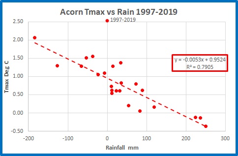
The BOM has sophisticated algorithms for area averaging temperature and rainfall across Australia and provide national climate records back to 1900 for rainfall and 1910 for maxima.  Averaged across Australia individual station idiosyncrasies are submerged so that the 1997 to 2019 relationship between Tmax and rainfall is very strong (and similar to that of Alice Springs):

Fig. 4: Tmax and Rainfall, Australia 1997-2019

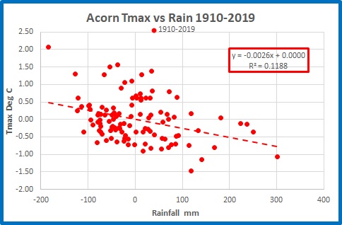
However, the relationship is not strong throughout the whole record:

Fig. 5: Tmax and Rainfall, Australia 1910-2019

The relationship from 1910 to 2019 is poor.

In the next figure I compare the Tmax – rainfall relationships for the first 10 years of the record with the last 10 years.

Fig. 6: Tmax and Rainfall, Australia, first and last decades

The trendlines are almost exactly parallel, with tight fits, showing strong relationships 100 years apart- but the trendline for 2010 to 2019 is about 1.7 degrees above that for 1910 – 1919.  How can that be?

It is possible to compare rainfall and temperature throughout the last 110 years.  In the next figure, rainfall is inverted and scaled down so as to match Tmax at 1910.

Fig. 7: Tmax and Inverted Scaled Rain, Australia

Running 10 year means allow us to see long term patterns of rainfall and temperature more easily:

Fig. 8: Tmax and Inverted Scaled Rain, Decadal Means, Australia

Rainfall has increased over the last 110 years (despite what you might hear in the media), and so apparently have maximum temperatures.  In the above figures Tmax and rainfall track roughly together until the mid-1950s, then Tmax takes off.

I calculated an “index” of temperature ~ rainfall variation by subtracting scaled, inverted rainfall from Tmax, commencing at zero in 1919.  This allows us to identify when temperature appears to diverge markedly from inverted rainfall:

Fig. 9: Index of Temperature ~ Rainfall Variation: Tmax minus Inverted Scaled Rain, Decadal Means, Australia

There is a small increase from the mid-1950s, but the really large divergence commences in the 1970s, with the decade from 1973 to 1982 about 0.6 units above the decade to 1972.  The index decreases to 1995, then there is another steep increase to 2007, and a final surge to 2019.

This index alone shows how poorly the official temperature record represents the temperature of the past.

 While there are other times, in the next figures I compare four periods: 1910 to 1972, 1973 to 1995, 1996 to 2007, and 2008 to 2019.  Here I use annual data.

Fig. 10: Tmax and Rainfall, Australia, four periods

Again, trendlines are almost parallel with similar slopes, showing that the Tmax ~ rainfall relationship is fairly constant for all periods- (about 0.5C per 100mm after 1995 and about 0.4C per 100mm before 1995).  However, the lines are separated.  Temperature for each later period is higher than the ones preceding, such that the temperature recorded now is about 1.5 degrees Celsius higher than it would have been for similar rainfall before 1973. And rainfall has increased in that time.

Global Warming Enthusiasts and apologists for the BOM will claim that these breaks between separate periods are real and caused by changes in circulation patterns due to climate change- in particular the Southern Annular Mode.  That will be the subject of Part 2.

Whatever the reasons, Australia wide the Tmax ~ rainfall relationship has remained constant for the past 110 years (as it should) but the temperatures reported in the Acorn dataset have increased by more than 1.5 degrees Celsius relative to rainfall.

Conclusion:

The ACORN-SAT temperature dataset is an unreliable record of Australia’s maximum temperatures.

CO2vid Watch: August

I have been wondering whether the largest real-life science experiment in history will show whether atmospheric carbon dioxide concentrations will decrease as a result of the Covid19-induced economic slowdown.

Earlier I concluded:  “I expect there may be a small decrease in the rate of CO2 concentration increase, but it won’t be much, and I will be surprised if it turns negative.  A large La Nina later this year will lead to a CO2 increase a few months later, in which case there will be a larger downturn in annual CO2 change in 2021.

However, if the major cause of CO2 increase is fossil fuel consumption, there will be an extra large decrease in CO2 change in 2020 and 2021- and a noticeable jump if the global economy rebounds.”

The CO2 concentration number for August is now published: 412.55 p.p.m. (parts per million).  The seasonal drawdown of CO2 has begun, but CO2 concentration is still 2.61 ppm above the figure for August last year.  Figure 1 shows the 12 month change in CO2 at Mauna Loa since 2015-that is, January to January, February to February, March to March.

Fig. 1:  12 month change in CO2 concentration since 2015 to August 2020- Mauna Loa

Figure 2 is a monthly update for 2020 I will show as each month’s CO2 figures become available (and 2021 if necessary):

Fig. 2:  Updated 12 month changes in CO2 concentration for 2020- Mauna Loa

Figure 3 shows the 12 month change in CO2 concentration since the record began.

Fig. 3:  12 month change in CO2 concentration since 1958 to August 2020- Mauna Loa

Annual growth has been above zero since the mid 1970s, and has not been below 1 ppm since 2011. The annual rate of change is increasing, in other words CO2 concentration growth is accelerating.

Note that so far this year, 12 month changes continue to remain firmly in the normal or even upper range, and there is no sign of any slow down. And there won’t be!

This paper by J. Reid explains why.

http://blackjay.net/?p=1021%20%3Chttp://blackjay.net/?p=1021%3E

CO2 growth appears to be an entirely natural process.

Unless something dramatic happens, I don’t think I will continue this series any longer. There’s nothing to see.

CO2vid Watch: July

I have been wondering whether the largest real-life science experiment in history will show whether atmospheric carbon dioxide concentrations will decrease as a result of the Covid19-induced economic slowdown.

Earlier I concluded:  “I expect there may be a small decrease in the rate of CO2 concentration increase, but it won’t be much, and I will be surprised if it turns negative.  A large La Nina later this year will lead to a CO2 increase a few months later, in which case there will be a larger downturn in annual CO2 change in 2021.

However, if the major cause of CO2 increase is fossil fuel consumption, there will be an extra large decrease in CO2 change in 2020 and 2021- and a noticeable jump if the global economy rebounds.”

The CO2 concentration number for July is now published: 414.38 p.p.m. (parts per million).  The seasonal drawdown of CO2 has begun, but CO2 concentration is 2.61 ppm above the figure for July last year.  Figure 1 shows the 12 month change in CO2 at Mauna Loa since 2015-that is, January to January, February to February, March to March.

Fig. 1:  12 month change in CO2 concentration since 2015 to July 2020- Mauna Loa

Notice the amount of 12 month change has increased a bit more.

Figure 2 is a monthly update for 2020 I will show as each month’s CO2 figures become available (and 2021 if necessary):

Fig. 2:  Updated 12 month changes in CO2 concentration for 2020- Mauna Loa

Note that so far this year, 12 month changes continue to remain firmly in the normal or even upper range, and there is no sign of any slow down.

Watch for next month’s update, and enjoy the ride!

CO2vid Watch: June

I have been wondering whether the largest real-life science experiment in history will show whether atmospheric carbon dioxide concentrations will decrease as a result of the Covid19-induced economic slowdown.

Earlier I concluded:  “I expect there may be a small decrease in the rate of CO2 concentration increase, but it won’t be much, and I will be surprised if it turns negative.  A large La Nina later this year will lead to a CO2 increase a few months later, in which case there will be a larger downturn in annual CO2 change in 2021.

However, if the major cause of CO2 increase is fossil fuel consumption, there will be an extra large decrease in CO2 change in 2020 and 2021- and a noticeable jump if the global economy rebounds.”

(In a coming post I will update my expectations for the end of the year and next year.) 

The CO2 concentration number for June is now published: 416.39 p.p.m. (parts per million).  The seasonal drawdown of CO2 has begun, but CO2 concentration is 2.47 ppm above the figure for June last year.  Figure 1 shows the 12 month change in CO2 at Mauna Loa since 2015-that is, January to January, February to February, March to March.

Fig. 1:  12 month change in CO2 concentration since 2015 to June 2020- Mauna Loa

Notice the amount of 12 month change has increased a little.

Figure 2 is a monthly update for 2020 I will show as each month’s CO2 figures become available (and 2021 if necessary):

Fig. 2:  Updated 12 month changes in CO2 concentration for 2020- Mauna Loa

Note that so far this year, 12 month changes are in the normal or even upper range, and there is no sign of any slow down.

Watch for next month’s update, and enjoy the ride!